Political activism in Greece
Political activism in ESS
Data
Read the data from the European Social Survey, round 4 (Greece).
For each of these survey questions, 1=“Yes” and 2=“No”.
-
contplt- Contacted politician or government official last 12 months -
wrkprty- Worked in political party or action group last 12 months -
wrkorg- Worked in another organisation or association last 12 months -
badge- Worn or displayed campaign badge/sticker last 12 months -
sgnptit- Signed petition last 12 months -
pbldmn- Taken part in lawful public demonstration last 12 months -
bctprd- Boycotted certain products last 12 months -
gndr- Gender -
agea- Age of respondent, calculated
ess_greece <- read_csv("https://daob.nl/files/lca/ess_greece.csv.gz")

ess_greece |> rmarkdown::paged_table()
Sadly, poLCA has no way of dealing with missing values other than “listwise deletion” (na.omit). For later comparability of models with different sets of variables, we create a single dataset without missings.
ess_greece <- na.omit(ess_greece)Show the data as pattern frequencies.
table(ess_greece) %>%
  as.data.frame() %>%
  filter(Freq != 0) %>%
  rmarkdown::paged_table()
Try out models with different number of classes
Create a convenience function that will fit the K-class model to the political participation data.
Apply the function to successively increasingly classes K = 1, 2, 3, …, 6. (Note: this can take a while!)
MK <- lapply(1:6, fitLCA)Compare model fit
Possible to look at AIC, BIC, etc.
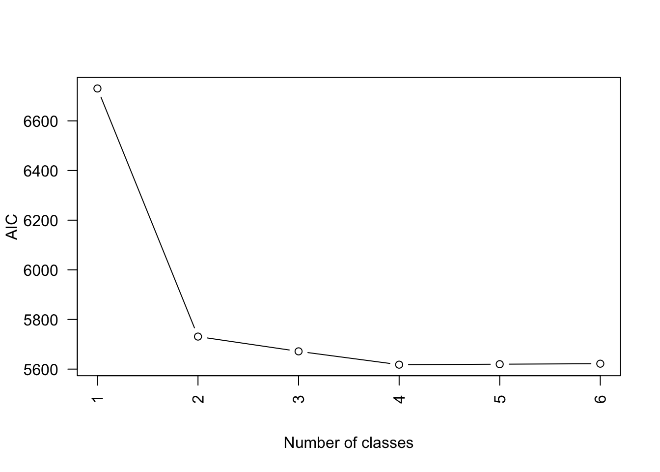

Select a model
We select the four-class model.
Here is the default plot given by polCA.
plot(fit)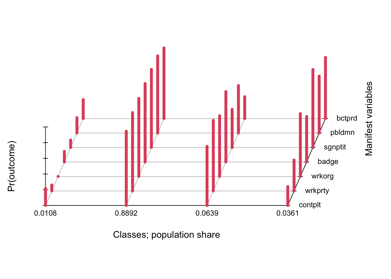
In this case the default plot is still somewhat readable, but in practice it is not the best as data visualizations go. A simple line plot does a better job (in my personal & completely subjective opinion!) and allows you to display confidence intervals to boot. We use tidy from the broom package to extract the results and ggplot to plot.
tidy(fit) %>% # from `broom` package
  filter(outcome == 2) %>%
  mutate(class = as.factor(class)) %>%
  ggplot(aes(variable, estimate, group = class, color = class)) +
  geom_point() + geom_line() +
  geom_errorbar(aes(ymin = estimate - 2*std.error,
                    ymax = estimate + 2*std.error), width = 0.2) +
  theme_bw() + scale_color_brewer(palette = "Set2")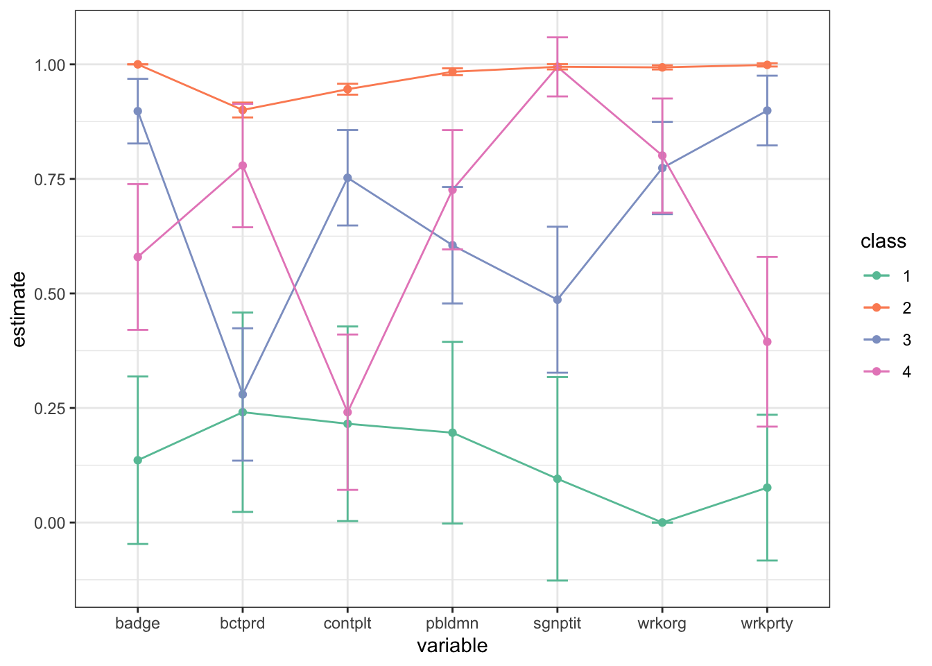
Local fit
library(poLCA.extras)

bvr(fit)
contplt wrkprty wrkorg badge sgnptit pbldmn
wrkprty 3.636971
wrkorg 5.427425 5.554144
badge 9.174424 11.568911 7.702777
sgnptit 3.027574 4.637158 4.743767 5.002371
pbldmn 2.748862 5.232943 6.068687 5.147027 3.224378
bctprd 3.042264 4.717105 5.596894 5.953936 2.472958 3.292210bootstrap_bvr_pvals(form_activism, fit, ess_greece, R = 200) contplt wrkprty wrkorg badge sgnptit pbldmn
wrkprty 1
wrkorg 1 1
badge 1 1 1
sgnptit 1 1 1 1
pbldmn 1 1 1 1 1
bctprd 1 1 1 1 1 1Classification quality
Create a data frame with the posterior class memberships and predicted class has the actual classification (predclass is the “modal assignment”)
Use the four-class model as the selected model
posteriors <- data.frame(post = fit$posterior,
                         predclass = fit$predclass)

classification_table <- posteriors %>%
  group_by(predclass) %>%
  summarize(across(starts_with("post."), ~ sum(.x)))

classification_table <- classification_table[,-1] |> as.matrix()

# Adopt the notation X=true latent class, W=assigned class
colnames(classification_table) <- paste0("X=", 1:4)
rownames(classification_table) <- paste0("W=", 1:4)

classification_table %>% round(1)
X=1 X=2 X=3 X=4
W=1 19.8 0.0 1.0 0.2
W=2 0.0 1822.0 34.8 11.1
W=3 1.1 7.5 87.4 3.0
W=4 1.4 4.0 8.6 60.1With column proportions:
classification_table |>
  prop.table(2) |>
  round(3)
X=1 X=2 X=3 X=4
W=1 0.887 0.000 0.008 0.003
W=2 0.000 0.994 0.264 0.149
W=3 0.051 0.004 0.663 0.040
W=4 0.062 0.002 0.065 0.808Entropy \(R^2\) and classification errors
Calculate classification errors from classification table:
Entropy \(R^2\):
Model with covariates
Now we fit the four-class model, but include covariates that predict the class membership. Class membership is predicted by gender and a quadratic age effect.
We also use the results from the model without covariates as starting values for the solution.
This is where the analyzed data would have been different if we had not already deleted all cases with at least one missing value above using na.omit. In practice this may lead to trouble, especially when there are many variables.
form_activism <- cbind(contplt, wrkprty, wrkorg,
                       badge, sgnptit, pbldmn, bctprd) ~
  gndr + agea + I(agea^2)

ess_greece_poly <- ess_greece %>%
  mutate(agea = scale(agea))

fit_covariates <-
  poLCA(form_activism,
        data = ess_greece_poly, nclass = 4,
        probs.start = fit$probs,
        verbose = FALSE, nrep = 50, maxiter = 3e3)
Warning in sqrt(diag(VCE.beta)): NaNs producedWarning in sqrt(diag(VCE.mix)): NaNs producedThe results now include multinomial regression coefficients in a model predicting class membership.
fit_covariatesConditional item response (column) probabilities,
by outcome variable, for each class (row)
$contplt
Pr(1) Pr(2)
class 1: 0.0521 0.9479
class 2: 0.5629 0.4371
class 3: 0.0857 0.9143
class 4: 0.7123 0.2877
$wrkprty
Pr(1) Pr(2)
class 1: 0.0011 0.9989
class 2: 0.5189 0.4811
class 3: 0.0046 0.9954
class 4: 0.5283 0.4717
$wrkorg
Pr(1) Pr(2)
class 1: 0.0041 0.9959
class 2: 0.6616 0.3384
class 3: 0.0537 0.9463
class 4: 0.2031 0.7969
$badge
Pr(1) Pr(2)
class 1: 0.0000 1.0000
class 2: 0.4844 0.5156
class 3: 0.0000 1.0000
class 4: 0.3946 0.6054
$sgnptit
Pr(1) Pr(2)
class 1: 0.0009 0.9991
class 2: 0.8837 0.1163
class 3: 0.1589 0.8411
class 4: 0.0000 1.0000
$pbldmn
Pr(1) Pr(2)
class 1: 0.0000 1.0000
class 2: 0.6053 0.3947
class 3: 0.2215 0.7785
class 4: 0.2538 0.7462
$bctprd
Pr(1) Pr(2)
class 1: 0.0686 0.9314
class 2: 0.7581 0.2419
class 3: 0.4770 0.5230
class 4: 0.2418 0.7582
Estimated class population shares
0.7934 0.0288 0.1345 0.0433
Predicted class memberships (by modal posterior prob.)
0.8589 0.0262 0.0776 0.0373
=========================================================
Fit for 4 latent classes:
=========================================================
2 / 1
Coefficient Std. error t value Pr(>|t|)
(Intercept) -0.66285 0.02401 -27.605 0.000
gndr -0.69438 0.22021 -3.153 0.002
agea -0.04689 0.01964 -2.387 0.019
I(agea^2) 0.00020 0.00029 0.701 0.485
=========================================================
3 / 1
Coefficient Std. error t value Pr(>|t|)
(Intercept) 0.40334 0.02398 16.816 0.000
gndr -0.41884 0.20307 -2.063 0.042
agea -0.04345 0.01840 -2.361 0.020
I(agea^2) 0.00016 0.00025 0.624 0.534
=========================================================
4 / 1
Coefficient Std. error t value Pr(>|t|)
(Intercept) -0.17721 0.04648 -3.813 0.000
gndr -0.84495 0.24730 -3.417 0.001
agea -0.06649 0.01986 -3.349 0.001
I(agea^2) 0.00066 0.00024 2.730 0.008
=========================================================
number of observations: 2062
number of estimated parameters: 40
residual degrees of freedom: 87
maximum log-likelihood: -2784.601
AIC(4): 5649.201
BIC(4): 5874.459
X^2(4): 148.8383 (Chi-square goodness of fit)
ALERT: iterations finished, MAXIMUM LIKELIHOOD NOT FOUND
ALERT: estimation algorithm automatically restarted with new initial values
The solution may have changed now that covariates are included.
tidy(fit_covariates) %>%
  filter(outcome == 2) %>%
  mutate(class = as.factor(class)) %>%
  ggplot(aes(variable, estimate, group = class, color = class)) +
  geom_point() + geom_line() +
  geom_errorbar(aes(ymin = estimate - 2*std.error,
                    ymax = estimate + 2*std.error), width = 0.2) +
  theme_bw() + scale_color_brewer(palette = "Set2")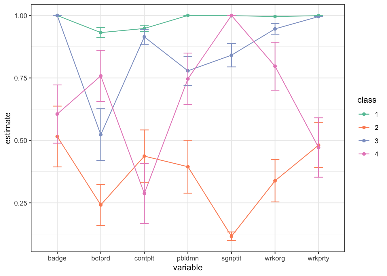
Effects plot
We can easily plot the results of the multinomial model using the effects library.
effect_age <- predictorEffects(fit_covariates, ~agea*gndr)
plot(effect_age, lines=list(multiline=TRUE))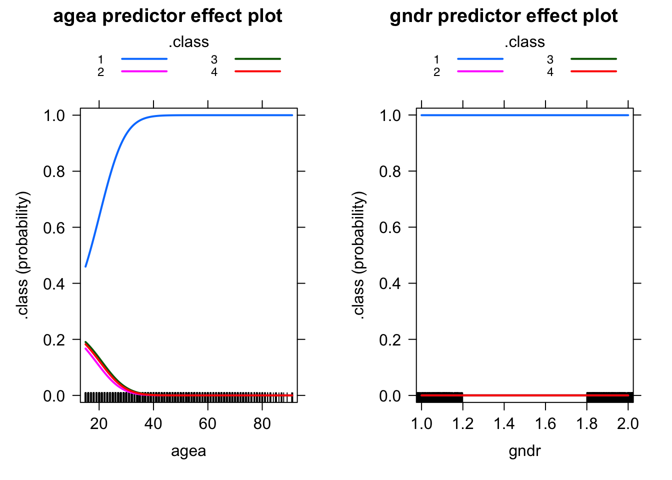
Three-step method using hand-rolled BCH weights
M <- prop.table(classification_table, 2)
Mi <- solve(M) # Weight matrix
K <- ncol(M) # Number of classes

# The data used by poLCA (may differ from raw due to missings):
dat_used_by_fit <- ess_greece
# Assigned class membership (by default uses modal assignment):
dat_used_by_fit$W <- fit$predclass
dat_used_by_fit$id_obs <- seq(NROW(dat_used_by_fit))

# Create expanded dataset with K rows for each observation:
ess_greece_expanded <- replicate(K, dat_used_by_fit, simplify = FALSE) |>
  reduce(rbind)

# Each of the replicated rows will correspond to one possible
#.  value of the true latent class:
ess_greece_expanded$X <- rep(1:K, each = NROW(dat_used_by_fit))

# Now we assign the BCH weights based on the
#.   inverse- misclassification matrix Mi
ess_greece_expanded <- ess_greece_expanded %>%
  mutate(w_bch = Mi[cbind(W, X)])

# Show a few rows of our constructed data:
ess_greece_expanded %>% arrange(id_obs) %>% head()
# A tibble: 6 × 13
contplt wrkprty wrkorg badge sgnptit pbldmn bctprd gndr agea W id_obs
<dbl> <dbl> <dbl> <dbl> <dbl> <dbl> <dbl> <dbl> <dbl> <int> <int>
1 2 2 2 2 2 2 1 2 37 2 1
2 2 2 2 2 2 2 1 2 37 2 1
3 2 2 2 2 2 2 1 2 37 2 1
4 2 2 2 2 2 2 1 2 37 2 1
5 2 2 2 2 2 2 1 2 26 2 2
6 2 2 2 2 2 2 1 2 26 2 2
# … with 2 more variables: X <int>, w_bch <dbl>The only library I was able to find that is both reliable and also does multinomial regression allowing negative weights is glmnet.
library(glmnet)

# We use glmnet with our BCH weights, w_bch, pretending X
#.  is observed. Set alpha and lambda =
fit_glmnet <- with(
  ess_greece_expanded %>% mutate(age_sq = agea^2),
  glmnet(cbind(gndr, agea, age_sq), X, weights = w_bch,
         family = "multinomial", alpha = 0, lambda = 0))

# The estimted coefficients
fit_glmnet |>
  coef() |>
  reduce(cbind) |>
  round(4)
4 x 4 sparse Matrix of class "dgCMatrix"
s0 s0 s0 s0
-0.8129 2.2496 -1.1247 -0.3119
gndr 0.0634 0.2132 -0.0632 -0.2134
agea -0.0081 -0.0256 0.0566 -0.0228
age_sq 0.0001 0.0003 -0.0008 0.0004# effects library does not work with glmnet so we have to roll
#. our own (again)
ef <- ess_greece %>%
summarize(agea = sort(unique(agea)),
age_sq = agea^2,
gndr = 1.5) %>%
bind_cols(predict(fit_glmnet, newx=as.matrix(.),
type = "response")[,,1])
names(ef)[4:7] <- paste0("X", 1:4)
# Show the effects plot
ef %>%
pivot_longer(X1:X4, names_to = "Class", values_to = "Prob") %>%
ggplot(aes(agea, Prob, colour = Class, group = Class)) +
geom_line() + theme_bw() +
scale_color_brewer(palette = "Set2")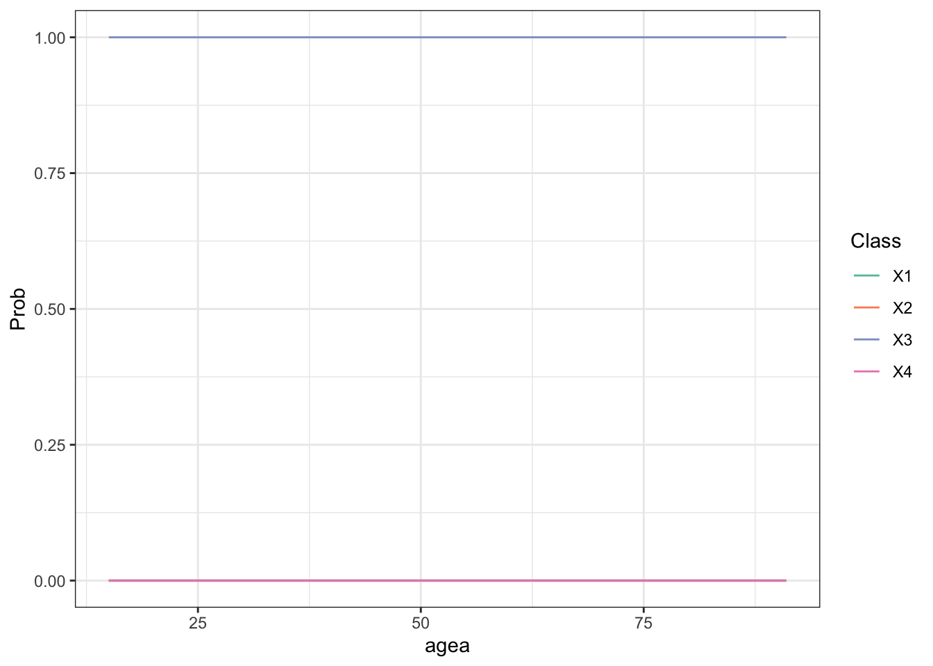
It gives results similar to those obtained with the one-step method.
SessionInfo
R version 4.2.2 (2022-10-31)
Platform: x86_64-apple-darwin17.0 (64-bit)
Running under: macOS Big Sur ... 10.16

Matrix products: default
BLAS:   /Library/Frameworks/R.framework/Versions/4.2/Resources/lib/libRblas.0.dylib
LAPACK: /Library/Frameworks/R.framework/Versions/4.2/Resources/lib/libRlapack.dylib

locale:
[1] en_US.UTF-8/en_US.UTF-8/en_US.UTF-8/C/en_US.UTF-8/en_US.UTF-8

attached base packages:
[1] stats     graphics  grDevices utils     datasets  methods   base

other attached packages:
 [1] glmnet_4.1-4         Matrix_1.5-1         effects_4.2-2
 [4] carData_3.0-5        poLCA.extras_0.1.0   poLCA_1.6.0.1
 [7] MASS_7.3-58.1        scatterplot3d_0.3-42 haven_2.5.1
[10] broom_1.0.1          forcats_0.5.2        stringr_1.5.0
[13] dplyr_1.0.9          purrr_0.3.4          readr_2.1.2
[16] tidyr_1.2.0          tibble_3.1.8         ggplot2_3.3.6
[19] tidyverse_1.3.2

loaded via a namespace (and not attached):
 [1] nlme_3.1-160        fs_1.6.1            lubridate_1.8.0
 [4] bit64_4.0.5         insight_0.19.0      RColorBrewer_1.1-3
 [7] httr_1.4.5          tools_4.2.2         backports_1.4.1
[10] utf8_1.2.3          R6_2.5.1            DBI_1.1.3
[13] colorspace_2.0-3    nnet_7.3-18         withr_2.5.0
[16] tidyselect_1.1.2    bit_4.0.5           curl_5.0.0
[19] compiler_4.2.2      cli_3.6.0           rvest_1.0.3
[22] xml2_1.3.3          labeling_0.4.2      scales_1.2.1
[25] digest_0.6.31       minqa_1.2.4         rmarkdown_2.16
[28] pkgconfig_2.0.3     htmltools_0.5.4     lme4_1.1-30
[31] dbplyr_2.2.1        fastmap_1.1.0       htmlwidgets_1.6.1
[34] rlang_1.0.6         readxl_1.4.1        rstudioapi_0.14
[37] shape_1.4.6         farver_2.1.1        generics_0.1.3
[40] jsonlite_1.8.4      vroom_1.5.7         googlesheets4_1.0.1
[43] magrittr_2.0.3      Rcpp_1.0.10         munsell_0.5.0
[46] fansi_1.0.4         lifecycle_1.0.3     stringi_1.7.12
[49] yaml_2.3.7          grid_4.2.2          parallel_4.2.2
[52] crayon_1.5.1        lattice_0.20-45     splines_4.2.2
[55] hms_1.1.2           knitr_1.40          pillar_1.8.1
[58] boot_1.3-28         codetools_0.2-18    reprex_2.0.2
[61] glue_1.6.2          evaluate_0.16       mitools_2.4
[64] modelr_0.1.9        foreach_1.5.2       vctrs_0.5.2
[67] nloptr_2.0.3        tzdb_0.3.0          cellranger_1.1.0
[70] gtable_0.3.0        assertthat_0.2.1    xfun_0.32
[73] survey_4.1-1        survival_3.4-0      googledrive_2.0.0
[76] gargle_1.2.0        iterators_1.0.14    ellipsis_0.3.2